Chapter 6 Data Visualization with Base Functions

We go through the base plotting functions in R in this chapter.

6.1 Scatter plot

Scatter plot is a good way to show the distribution of data points.

data(mtcars)
plot(mtcars$mpg, mtcars$wt) # with first as x, and second as y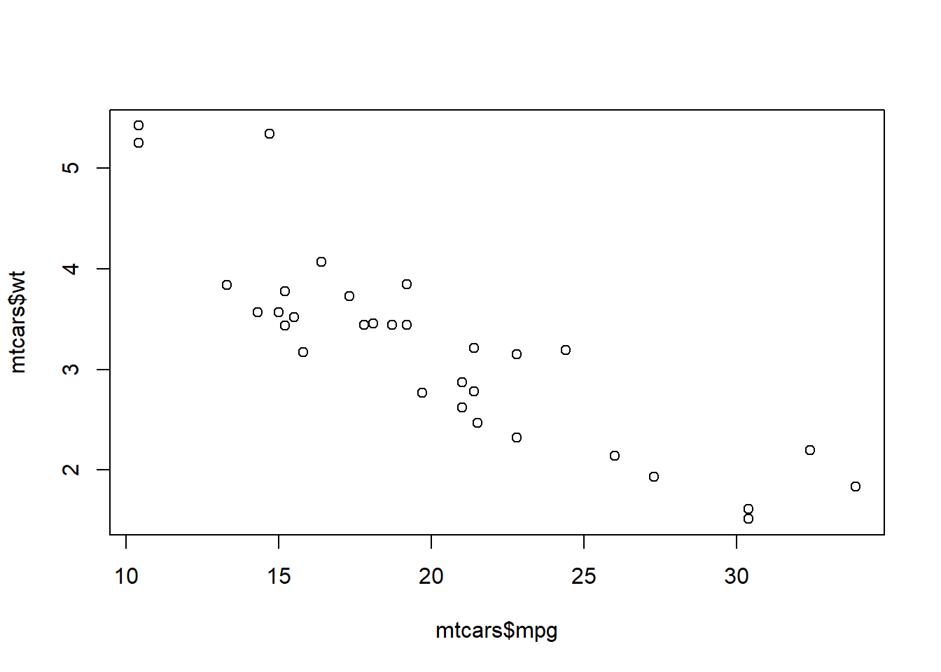

Or, you could use the variable names directly and indicate the dataset as the codes below. You will get the same result.

plot(wt ~ mpg, data = mtcars) # you have to specify the name of the data frame here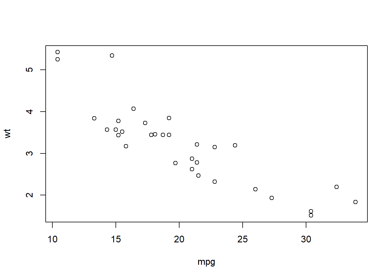

6.2 Line plot

You could transfer the scatter plot above to a line plot by just adding a type variable to indicate that you are plotting a line. Line plot is good for presenting the trend of a variable changing by time.

year <- c(1998:2003) # create variable year
sales <- c(500, 600, 650, 700, 400, 550) # create variable sales
df <- data.frame(year, sales) # combine the variables into one data frame called df

plot(sales ~ year, data = df,
     type = 'l') # type indicates the line type with l

You could also choose another type by changing the value of type, as the one below.

plot(sales ~ year, data = df,
     type = 'b') # b for both line and pint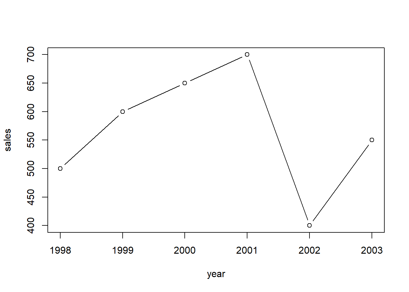

You could use help(plot) to check more styles of the plots.

6.3 Bar plot

Bar plot is a good way to compare the values in each year or for each item. You could use barplot() to draw it.

barplot(df$sales,
        names.arg = df$year) # names.org indicates the vector of names to be plotted under each bar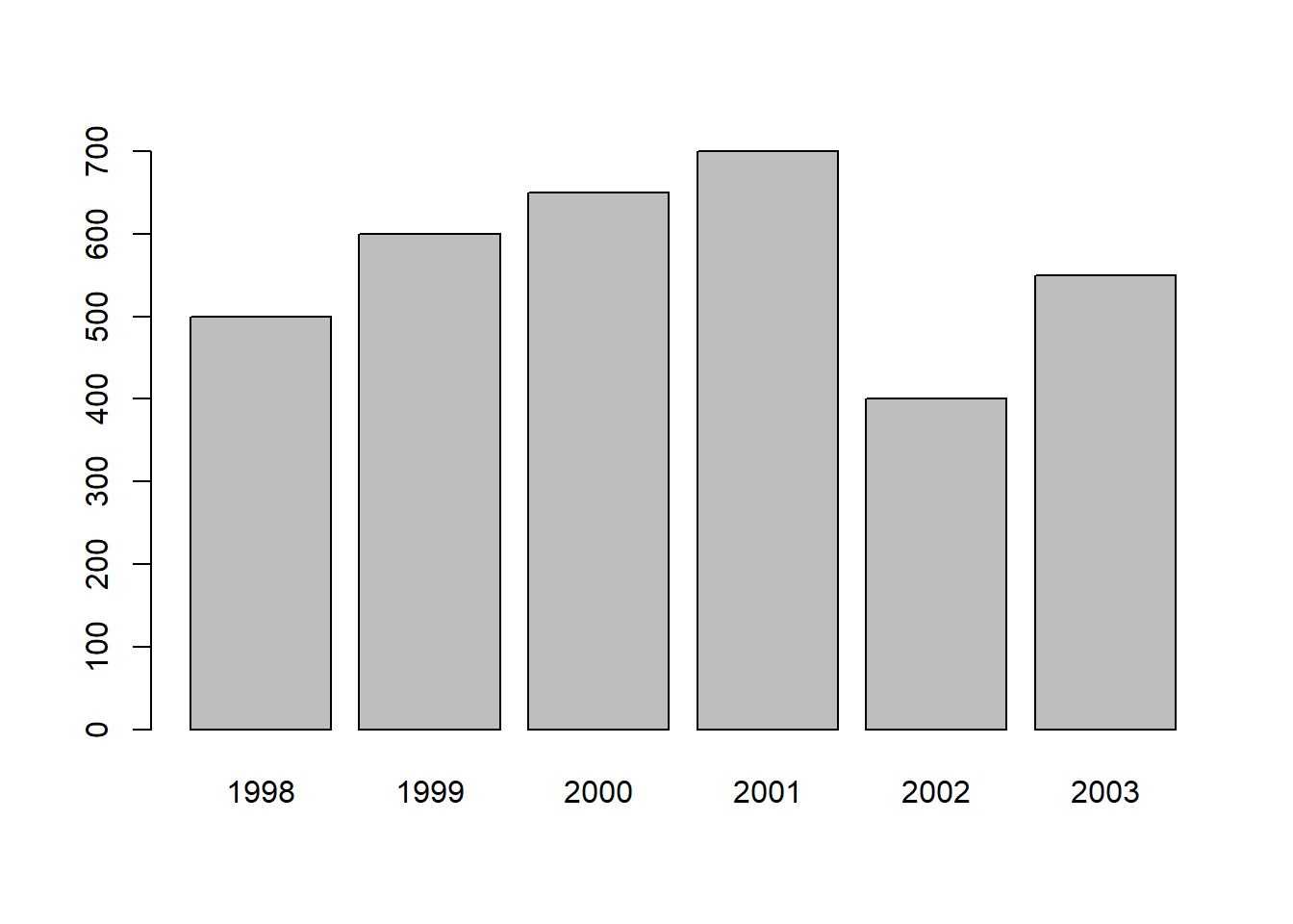

6.4 Add more elements in the plots

For a reader-friendly plots, you have to add more information such as title, labels, and legend. For the plot above, we could use the codes below to make it more informative.

barplot(df$sales,
        names.arg = df$year,
        main = 'Bar plot of the sales for each year from 1998 to 2003', # add title for the plot
        xlab = 'Year', # add label tag for the x-axis
        ylab = 'Sales (million dollors)',  # add label for the y-axis
        ylim = c(0, 1000), # set the range of y axis, you could set the range of x axis with xlim
        legend = 'Sales') # add legend name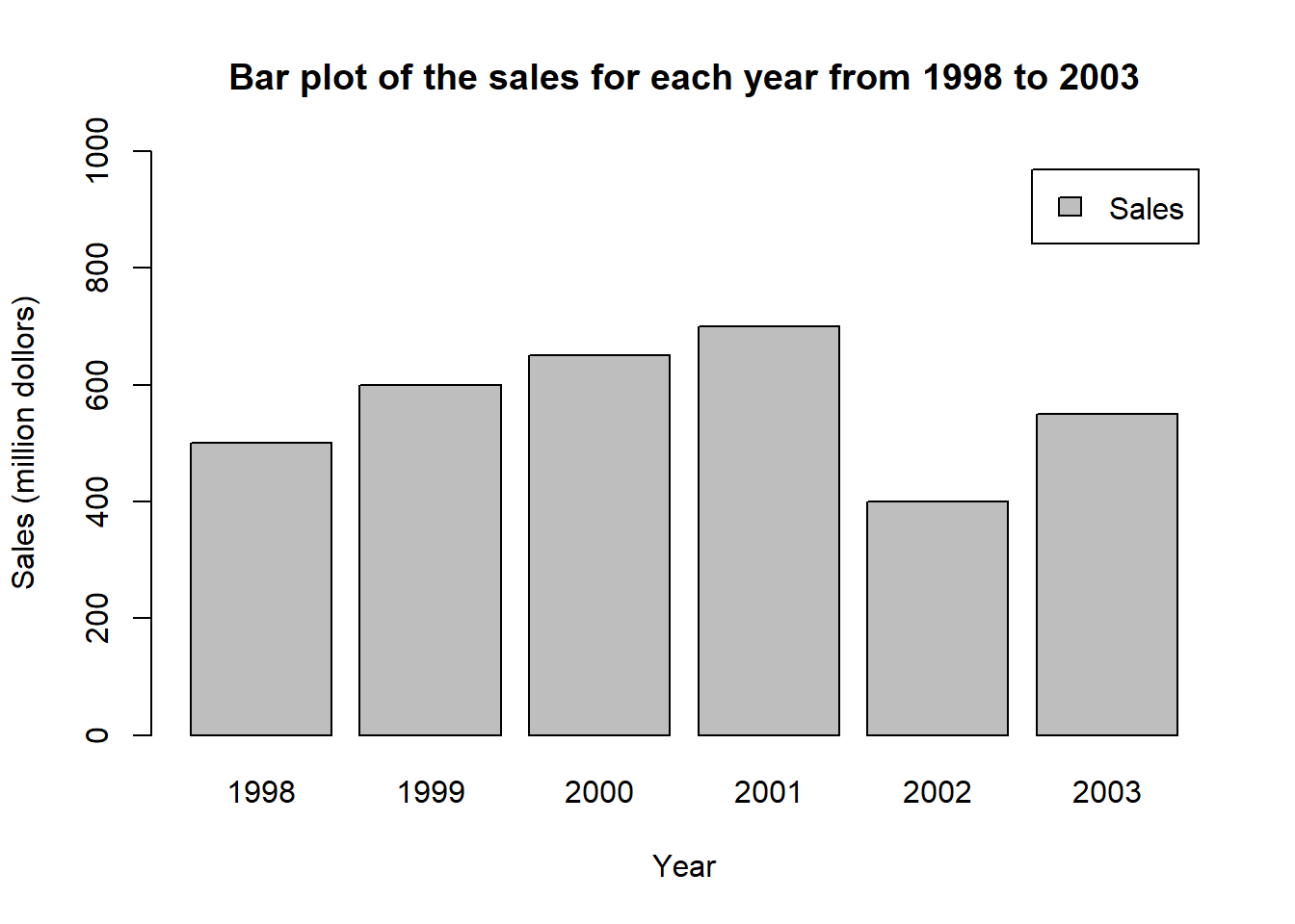

6.5 Pie chart

Pie chart is a good way to show the share of each part. You could use pie() function to draw a pie chart in R.

pie(df$sales, # value for each piece
    labels = df$year, # label for each piece
    main="Pie Chart of the Sales in ecah Year")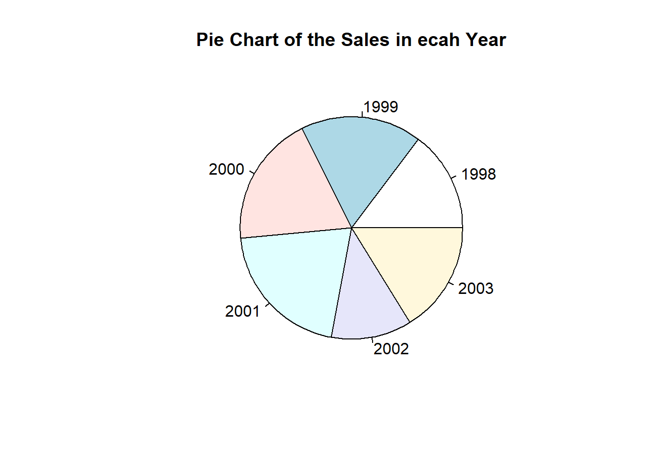

6.6 Boxplot

Boxplot is also called box-whisker plot. It is to present the distribution of the dataset based on their quartiles. In R, you could use boxplot() to draw a boxplot.

t <- c(1, 5, 10, 7, 8, 10, 11, 19)
boxplot(t, range = 0) # set range = 0 makes the whiskers reach the samllest and largest values in the dataset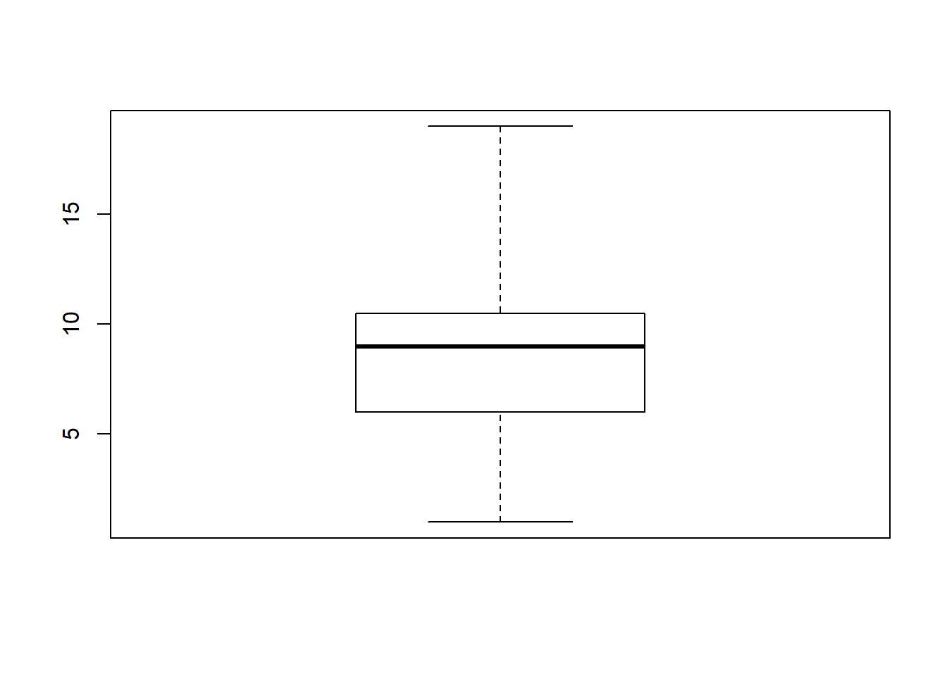

t <- c(1, 5, 10, 7, 8, 10, 11, 19)
boxplot(t, range = 1) # set range = 1 makes the the whiskers extend to the most extreme data point which is no more than range times the interquartile range from the box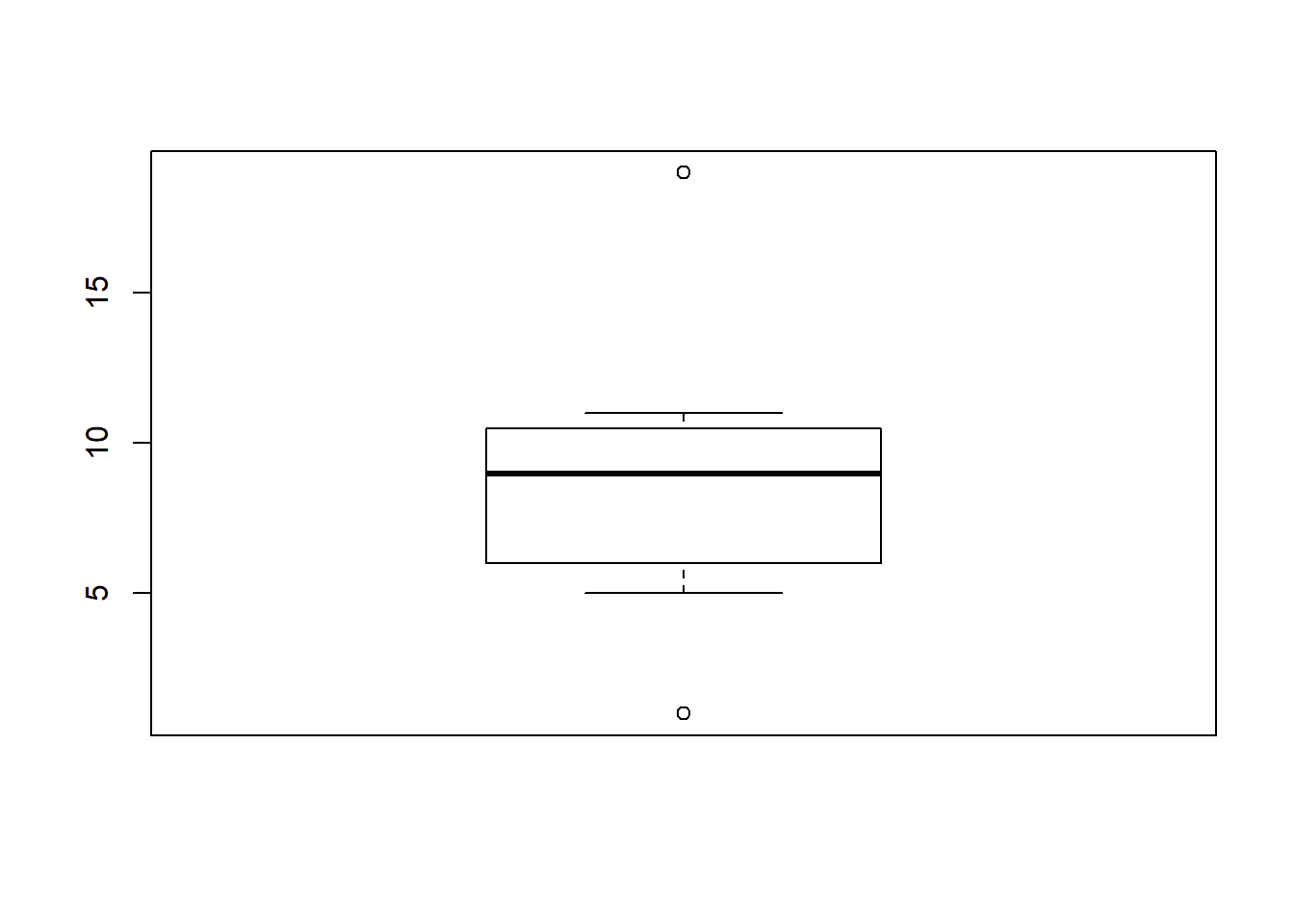

6.7 Color in R

You could change the color of the plots by adding col = in the functions. For example.

plot(sales ~ year, data = df,
     type = 'b',
     col = 'YellowGreen') # specify the name of the color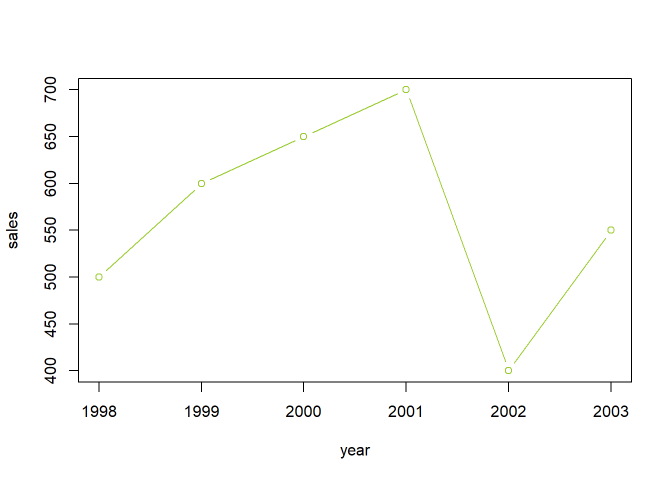

Here is a link where you could find the name of the color.

You could also use the hexadecimal color code to indicate the color. For example.

barplot(df$sales,
        names.arg = df$year,
        main = 'Bar plot of the sales for each year from 1998 to 2003', 
        xlab = 'Year', 
        ylab = 'Sales (million dollors)',  
        legend = 'Sales',
        col = '#009999') # use the hexadecimal color code, you need to start it with the hash tag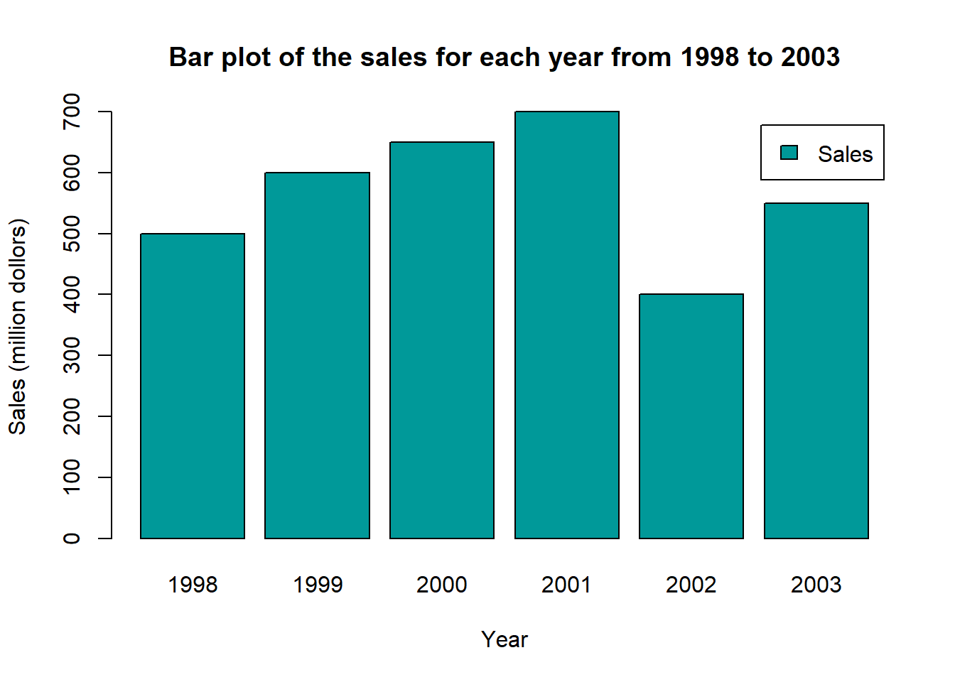

By the same link, you could also find the hexadcimal code for each color.