Chapter 9 Spatial Data Visualization

In this chapter, we will learn how to deal with the geospatial dataset with packages sf. We will also interact it with ggplot2. Link for the slides of this lecture.

9.1 Why spatial visualization with R?

The common solutions for creating maps include GIS (Geographic Information System) software: ArcGIS, QGIS, etc. They are powerful in spatial data visualization and analysis. However, they do have some disadvantages, such as the workflow is not easy to reproduce, not good at statistical computing, etc. As R has more and more powerful packages that could deal with geospatial data, many researchers and practitioners start to use R in their work. Comparing ArcGIS (or QGIS) with R, is similar with comparing Stata with R. Both of them have pros and cons. Whether or not you use them depends on your personal preference and task requirements.

Then when we should use R to do spatial data visualization, not ArcGIS? Well, one situation is that you do not have access to ArcGIS (ArcGIS is not free), then R is a good choice for you. Another situation could be that you have used R for your data analysis and then you could continue to use R to do spatial visualization. You do not need to change the working environment in this case. Or if you want to make your work more reproducible, R is a good choice since its codes can be recycled for other similar work and you could check your codes to track your data analysis history.

9.2 Some basics about spatial data

Spatial data has some differences with our common data. The largest one is that it has spatial attributes for indicate locations. Those spatial attributes could be points, lines, or/and ploygon. It could also be the combination of these elements. Points could be the positions for a single-family house, an intersection, a bar, etc. Lines could be the segments streets, rivers, etc. Polygons could be the boundaries states, counties, cities, etc. As shown in the figure below Source. While they are different spatial attributes, they are all combined with points.

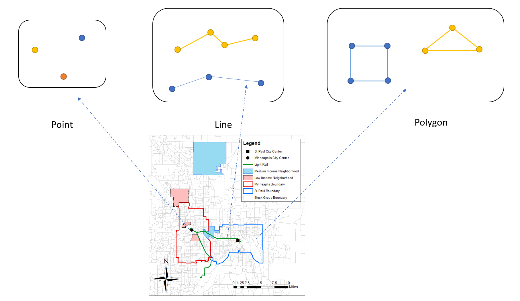
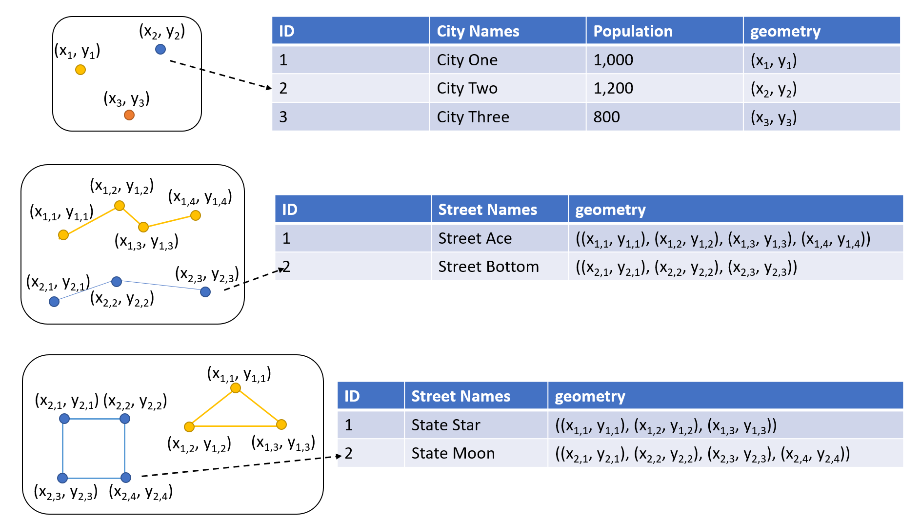
For a spatial data file in R, it is similar to the common dataset. It is a 2-D table with each column for a variable. The spatial data also has a column called geometry. This is the variable indicating the spatial attributes. For example, for a spatial file including the points of several cities in Minnesota. Its geometry column will be the longitudes and latitudes of those points. If a spatial file contains the boundaries of the states in the U.S., then its geometry column will be the locations of the polygons. If a spatial data has the information of points, it is called point spatial data. If a spatial data has the information of lines, it is called line spatial data. If a spatial data has the information of polygons, it is called polygon data. A spatial data file can only include one type of spatial attribute.

For all geospatial variables, they should have a very important information called coordinate reference system (CRS). We will not expand the concept in this lecture. The simple idea is that it is the system to locate geographical entities. For example, you could use longitude and latitude to locate the position of everything on earth, which is a 3D sphere. Or you could use another type of CRS to locate the position of something in a 2D flattened map, as shown in the figure below (Source). For the a same position, its indice will be different in different CRSs. There are two formats of CRS. One is EPSG and the other is proj4string. EPSG is a combination of numbers. proj4string contains variables and values. You could find more information about them in this link.

After reviewing some concepts for geospatial data. Let’s write some codes in R.

Before start, let’s install the package first.

install.packages('sf')

And import the package.

library(sf)

## Linking to GEOS 3.8.0, GDAL 3.0.4, PROJ 6.3.1

9.3 Read files

The file format to store the spatial data is shapefile. We could import the shapefile with st_read() function into R.

The dataset is from the Minnesota Geospatial Commons. It contains the geospatial information of the census tracts of the Twin Cities metro area.

map <- st_read('Census2010RealignTract.shp')

## Reading layer `Census2010RealignTract' from data source `C:\UMN\Course\R_course\PA5928-Data-management-and-visualization-with-R\Census2010RealignTract.shp' using driver `ESRI Shapefile'
## Simple feature collection with 708 features and 10 fields
## geometry type:  POLYGON
## dimension:      XY
## bbox:           xmin: 419967.5 ymin: 4924224 xmax: 521254.7 ymax: 5029010
## projected CRS:  NAD83 / UTM zone 15N

After running the codes, the console has shown some information about the shapefile we just read.

class(map)

## [1] "sf"         "data.frame"

With class(), we could check the type of the variable. It is both sf and data.frame. sf means the dataset is a type of geospatial data and contains some related information. data.frame means that the dataset is also a data frame and could be managed by many functions working on data frames.

head(map)

## Simple feature collection with 6 features and 10 fields
## geometry type:  POLYGON
## dimension:      XY
## bbox:           xmin: 427577.5 ymin: 4924224 xmax: 516478.2 ymax: 4949418
## projected CRS:  NAD83 / UTM zone 15N
##   TRACT STATE  CO TRACTCE10       GEOID   ALAND10 AWATER10    Acres Shape_Leng
## 1 61502    27 037    061502 27037061502 149642919  4668565 38134.50   54449.32
## 2 61402    27 037    061402 27037061402 211963640  3786753 53258.86   66036.81
## 3 81200    27 139    081200 27139081200  90667239  3288582 23205.13   38782.40
## 4 61501    27 037    061501 27037061501 168761402  1932931 42132.88   65971.67
## 5 81100    27 139    081100 27139081100 183756089  3059699 46115.82   58071.16
## 6 81300    27 139    081300 27139081300 218177258  3688572 55189.04   94116.03
##   Shape_Area                       geometry
## 1  154324840 POLYGON ((477636.4 4932330,...
## 2  215530975 POLYGON ((496883.5 4929115,...
## 3   93907812 POLYGON ((448700 4932487, 4...
## 4  170505702 POLYGON ((496863.3 4932245,...
## 5  186624108 POLYGON ((458497.9 4932388,...
## 6  223342132 POLYGON ((439064.1 4943284,...

With head(), we could see that there is a column called geometry. Every sf file will have this column, where stores the geospatial information of the observations. Other columns are just normal columns containing information for the observations.

We could use st_crs() to check the CRS of the variable.

st_crs(map)

## Coordinate Reference System:
##   User input: NAD83 / UTM zone 15N 
##   wkt:
## PROJCRS["NAD83 / UTM zone 15N",
##     BASEGEOGCRS["NAD83",
##         DATUM["North American Datum 1983",
##             ELLIPSOID["GRS 1980",6378137,298.257222101,
##                 LENGTHUNIT["metre",1]]],
##         PRIMEM["Greenwich",0,
##             ANGLEUNIT["degree",0.0174532925199433]],
##         ID["EPSG",4269]],
##     CONVERSION["UTM zone 15N",
##         METHOD["Transverse Mercator",
##             ID["EPSG",9807]],
##         PARAMETER["Latitude of natural origin",0,
##             ANGLEUNIT["Degree",0.0174532925199433],
##             ID["EPSG",8801]],
##         PARAMETER["Longitude of natural origin",-93,
##             ANGLEUNIT["Degree",0.0174532925199433],
##             ID["EPSG",8802]],
##         PARAMETER["Scale factor at natural origin",0.9996,
##             SCALEUNIT["unity",1],
##             ID["EPSG",8805]],
##         PARAMETER["False easting",500000,
##             LENGTHUNIT["metre",1],
##             ID["EPSG",8806]],
##         PARAMETER["False northing",0,
##             LENGTHUNIT["metre",1],
##             ID["EPSG",8807]]],
##     CS[Cartesian,2],
##         AXIS["(E)",east,
##             ORDER[1],
##             LENGTHUNIT["metre",1]],
##         AXIS["(N)",north,
##             ORDER[2],
##             LENGTHUNIT["metre",1]],
##     ID["EPSG",26915]]

Luckily, this variable contains the right CRS. For the maps in the area of Minnesota, the CRS is the one showing above, 26915 for EPSG.

However, sometimes, the file does not have CRS information. You have to check the original source of the file and assign the right CRS to it.

st_crs(map) <- 26915

By doing this, there is a message telling that this function will not do the transformation for us. Sometimes, even if the file contains the right CRS, its CRS might be different from other files. If you want to map them in the same page or want to do geospatial data analysis among them, you have to transfer the CRSs of them to the same one. You could do this by using st_transform().

We could use ggplot2 to visualize the map. For simply mapping the polygons, we do not need to specify aes(). And we use geom_sf() to plot map.

library(ggplot2)

ggplot(map) +
  geom_sf()

9.4 Deal with spatial data like data frame

As the spatial data is also a data frame in R. We could use dplyr to deal with it. For example, select the column we want.

The current spatial data map contains some variables we do not need, so we could select the useful ones by using select() function in dplyr. Please pay attention that we do not need to select the geometry column. It will be selected automatically. In this lecture, we only select GEOID, which is the ID for each area/tract.

library(dplyr)
new_map <- map %>%
  select(GEOID)

We could join other data to the current geospatial variable by the join functions in dplyr. Firstly, we import the data.

library(readr)
data <- read_csv('data.csv')

## 
## -- Column specification --------------------------------------------------------
## cols(
##   GEOID = col_double(),
##   POPTOTAL = col_double(),
##   HHTOTAL = col_double(),
##   AGEUNDER18 = col_double(),
##   AGE18_39 = col_double(),
##   AGE40_64 = col_double(),
##   AGE65UP = col_double()
## )

This dataset also has a variable called GEOID, which could be used to do the join operation. The list below presents the descriptions of other variables, which are all from 2012-2016 five-year ACS estimates.

Variable	Descriptions
GEOID	Unique identifier used by Census FactFinder website
POPTOTAL	Total population
HHTOTAL	Total households
AGEUNDER18	Population age under 18
AGE18_39	Population in this range
AGE40_64	Population in this range
AGE65UP	Populationage 65+

class(new_map$GEOID)

## [1] "factor"

class(data$GEOID)

## [1] "numeric"

We could join this data to the map by using the GEOID column. Before join operation, we have to transfer the GEOID to match the data type of GEOID in the map file. Currently, their types are different, one is factor and other is numeric. They have to be the same data type before joining.

data <- data %>%
  mutate(GEOID = factor(GEOID))

Then, we do the join operation.

new_map <- new_map %>%
  left_join(data, by = 'GEOID')

This message tells us that the levels of factors in the GEOIDs of the two files are different. This makes sense, since the data file has more observations, which also will have more levels.

9.5 Data management

We calculate the percentage of old people in each census tract.

new_map <- new_map %>%
  mutate(old_percent = AGE65UP/POPTOTAL)

9.6 Spatial data visualization

We could use ggplot2 by its geom_sf() function.

p <- ggplot(new_map, aes(fill = old_percent)) + # use fill to indicate the variable you want to visualize
  geom_sf()
p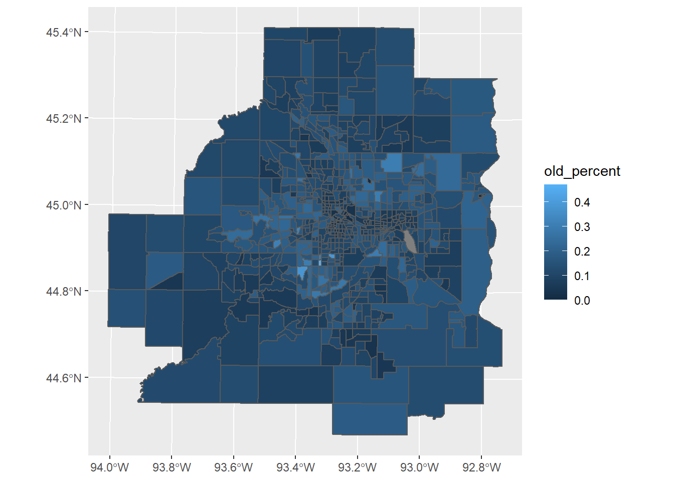

The color is not good, we could add scale_fill_gradient() to specify the colours we want.

p + scale_fill_gradient(low = 'white', high = 'red')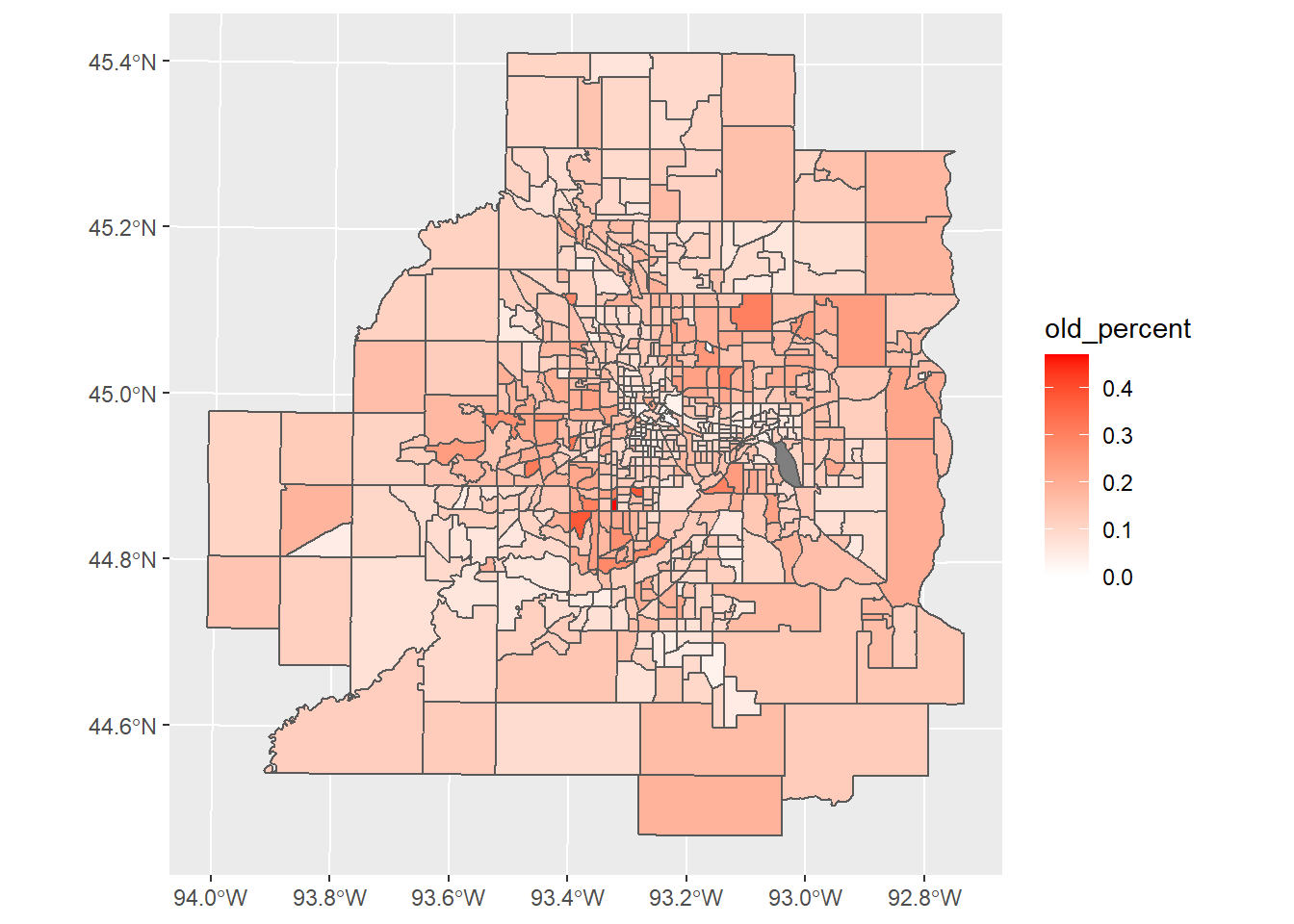

Again, we could add more information to make the figure better and more readable, and change the theme a little bit.

p + scale_fill_gradient(low = 'white', high = 'red') +
  labs(title = 'Distribution of old population in the Twin Cities area',
       fill = 'Percentage') +
  theme_bw()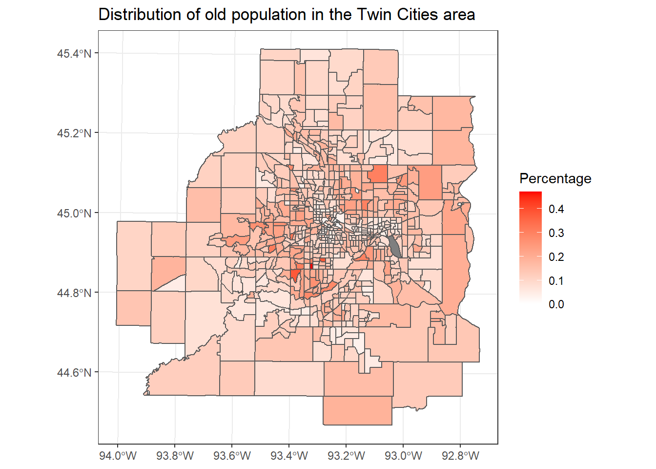

Finally, we could use ggsave() to save the plot we want after we run the ggplot() function.

9.7 More example

We could visualize the population directly in the map with ggplot2.

ggplot(new_map, aes(fill = POPTOTAL)) +
  geom_sf(colour = 'White') +
  scale_fill_gradient(low = 'white', high = 'Orange') +
  labs(title = 'Distribution of population in the Twin Cities area',
       fill = 'Population') +
  theme_bw()

9.8 Add other layers to the current plot

We could add other layers to the current plot. We import the spatial data of the transit routes in the metro area.

transit_route <- st_read('TransitRoutes.shp')

## Reading layer `TransitRoutes' from data source `C:\UMN\Course\R_course\PA5928-Data-management-and-visualization-with-R\TransitRoutes.shp' using driver `ESRI Shapefile'
## Simple feature collection with 227 features and 32 fields
## geometry type:  MULTILINESTRING
## dimension:      XY
## bbox:           xmin: 409591 ymin: 4947433 xmax: 515317.7 ymax: 5046090
## projected CRS:  NAD83 / UTM zone 15N

We add the transit route layers to the current plot by adding one more geom_sf().

ggplot(new_map) +
  geom_sf() +
  geom_sf(data = transit_route)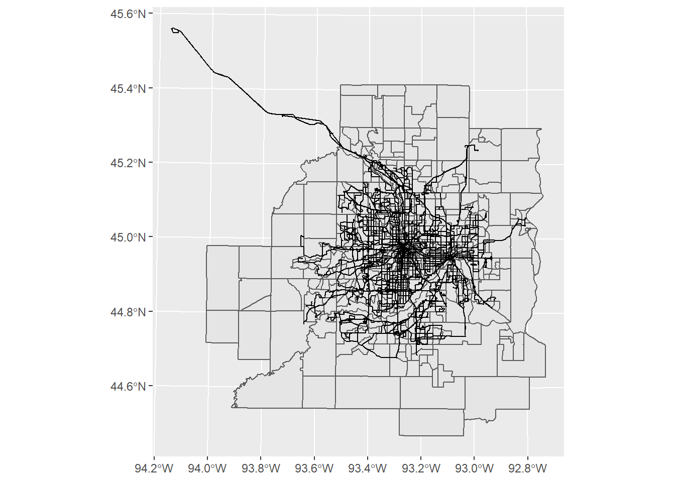

Add titles and themes to it.

ggplot(new_map) +
  geom_sf(fill = NA, colour = 'Grey') +
  geom_sf(data = transit_route, colour = 'Blue') +
  labs(title = 'Transit route in the Twin Cities Metro area') +
  theme_bw()

9.9 Geospatial data analysis

For those who are familiar with geospatial operations in ArcGIS, sf also provides functions to do geospatial data analysis, such as spatial join, intersect, clip, etc. For example, you could use st_join() to carry out spatial join, use st_intersects() to do intersect, and st_intersection() to do clip. You could find more here.