Chapter 5 Data Manipulation with dplyr
In this chapter, we will learn a very popular package dplyr to deal with data manipulation. We will mainly go through its main functions (BiomedicalDataScience 2019; r-project 2019).
5.1 select()
Before the lecture, install the package in your computer.
install.packages('dplyr') ## you only need to install this package onceLet’s first import this package. Also, we import the Minneapolis ACS dataset.
library(dplyr)
minneapolis <- read.csv('minneapolis.csv')
If we want to select one or more columns (i.e., variables) from the dataset. We could use select() in dplyr. It is similar to subset() , but here, you do not need to use select = c('mpg', 'disp'). You use the names of the columns directly in the function.
df <- select(minneapolis, # name of the data frame
       YEAR, SEX, AGE) # column/variable names you want to select
head(df, 3)
## YEAR SEX AGE
## 1 2010 2 59
## 2 2010 2 29
## 3 2010 1 54You could also use the index of the columns.
df <- select(minneapolis, # name of the data frame
       c(1:3)) # index of the columns/variables you want to select
head(df, 3)
## YEAR SEX AGE
## 1 2010 2 59
## 2 2010 2 29
## 3 2010 1 54pipe
The codes above is kind of a traditional way to do the work. We start with a function and put parameters in the function. However, this is not the typical way to use dplyr.
The codes below is a more dplyr way people use the package. We start with the name of the data frame. Then, we put a special sign %>% called pipe after it. We continue from a new line and write the function we want to use. Besides that, we could add more functions with the pipe operator. For example, only show first three observations with head().
minneapolis %>% # name of the data frame
  select(YEAR, SEX, AGE) %>% # select the columns by their names
  head(3)
## YEAR SEX AGE
## 1 2010 2 59
## 2 2010 2 29
## 3 2010 1 54The original codes include more (see below). When comparing the codes above and below, you will find that original codes use . as the input of the data frame in the function. However, for easy coding, this . could be omitted if it is in the starting position among the input parameters in the functions. In other words, if this . is not in the starting position, it cannot be omitted.
minneapolis %>%
  select(., YEAR, SEX, AGE) %>%
  head(., 3)
## YEAR SEX AGE
## 1 2010 2 59
## 2 2010 2 29
## 3 2010 1 54You can also write the codes in only one line, just like the codes below. However, it is recommended to write codes with one function in one line to improve the readiness of the codes.
minneapolis %>% select(YEAR, SEX, AGE) %>% head(3)## YEAR SEX AGE
## 1 2010 2 59
## 2 2010 2 29
## 3 2010 1 54The pipe operation is named after the art work, This is not a pipe, from René Magritte.

We will keep using the fashion of pipe in the following lectures. In addition, you can use Ctrl + Shift + M in RStudio to quickly input the pipe operator.
Besides selecting some columns you want, you could also exclude the columns you do not want by putting a negative sign - before the variable.
minneapolis %>%
  select(-HISPAN, - FTOTINC) %>% ## exclude HISPAN and FTOTINC from the data frame
  head(3)
## YEAR SEX AGE RACE EDUC EMPSTAT INCTOT
## 1 2010 2 59 1 10 1 33100
## 2 2010 2 29 1 10 1 16000
## 3 2010 1 54 2 7 3 1100You could use : to select a range of variables.
minneapolis %>%
  select(YEAR:RACE) %>% # select from YEAR to RACE in the data frame
  head(3)
## YEAR SEX AGE RACE
## 1 2010 2 59 1
## 2 2010 2 29 1
## 3 2010 1 54 2Or exclude a range of variables.
minneapolis %>%
  select(-(YEAR:RACE)) %>% # exclude the variables from YEAR to RACE in the data frame
  head(3)
## HISPAN EDUC EMPSTAT INCTOT FTOTINC
## 1 0 10 1 33100 49100
## 2 0 10 1 16000 49100
## 3 0 7 3 1100 NABelow are some advanced techniques to select columns.
You can select the column with their names starting with the string(s) you specify in starts_with(). For example, the codes below select the columns with names starting with E.
minneapolis %>%
  select(starts_with('E')) %>%
  head(3)
## EDUC EMPSTAT
## 1 10 1
## 2 10 1
## 3 7 3It may not make sense to you at first. I apologize that the example above is not a good one. In my experience, I have dealt with a traffic dataset that contains variables such as AADT_2010, AADT_2011, AADT_2012, AADT_2013, AADT_2014, AADT_2015. In this case, you can use codes like select(starts_with('AADT')) to select all similar columns.
Since we have starts_with(), you may be wondering it there is ends_with(). The answer is yes.
minneapolis %>%
  select(ends_with('E')) %>%
  head(3)
## AGE RACE
## 1 59 1
## 2 29 1
## 3 54 2You can use contains() to select the columns containing the string(s) you specify.
minneapolis %>%
  select(contains('INC')) %>%
  head(3)
## INCTOT FTOTINC
## 1 33100 49100
## 2 16000 49100
## 3 1100 NAOther similar functions include num_range(), matches(), one_of(), etc. Feel free to check how they can be used with help().
5.2 filter()
In dplyr, we use filter() to select the rows satisfying some conditions.
minneapolis %>%
  filter(YEAR == 2015) %>%
  head(3)
## YEAR SEX AGE RACE HISPAN EDUC EMPSTAT INCTOT FTOTINC
## 1 2015 2 37 3 0 11 1 125000 125000
## 2 2015 1 18 1 0 6 3 2500 NA
## 3 2015 1 91 1 0 6 3 8400 NAAdd more conditions by using , to separate them.
minneapolis %>%
  filter(YEAR == 2015,
         AGE == 37,
         SEX == 1) %>%
  head(3)
## YEAR SEX AGE RACE HISPAN EDUC EMPSTAT INCTOT FTOTINC
## 1 2015 1 37 1 0 7 1 55000 75000
## 2 2015 1 37 1 0 6 1 40000 73600
## 3 2015 1 37 1 0 7 1 80000 80000minneapolis %>%
filter(YEAR == 2015,
INCTOT > mean(INCTOT, na.rm = T)) %>% ## select those with an above-average personal income
head(3)## YEAR SEX AGE RACE HISPAN EDUC EMPSTAT INCTOT FTOTINC
## 1 2015 2 37 3 0 11 1 125000 125000
## 2 2015 2 42 1 0 11 1 160200 270400
## 3 2015 1 42 1 0 10 1 110200 270400, serves as an logical and here. Instead, you can use &.
minneapolis %>%
  filter(YEAR == 2015 & INCTOT > mean(INCTOT, na.rm = T)) %>%
  head(3)
## YEAR SEX AGE RACE HISPAN EDUC EMPSTAT INCTOT FTOTINC
## 1 2015 2 37 3 0 11 1 125000 125000
## 2 2015 2 42 1 0 11 1 160200 270400
## 3 2015 1 42 1 0 10 1 110200 270400You may use | to stand for logical or.
minneapolis %>%
  filter(YEAR == 2015 | YEAR == 2017) %>% ## select those in 2015 or 2017
  head()
## YEAR SEX AGE RACE HISPAN EDUC EMPSTAT INCTOT FTOTINC
## 1 2015 2 37 3 0 11 1 125000 125000
## 2 2015 1 18 1 0 6 3 2500 NA
## 3 2015 1 91 1 0 6 3 8400 NA
## 4 2015 2 18 1 0 6 1 1000 NA
## 5 2015 1 19 1 0 6 3 3000 NA
## 6 2015 2 18 1 0 6 1 3300 NA5.3 arrange()
We could arrange the order of some columns by arrange() functions.
minneapolis %>%
  arrange(YEAR) %>% # arrange YEAR in ascending order
  head(5)
## YEAR SEX AGE RACE HISPAN EDUC EMPSTAT INCTOT FTOTINC
## 1 2010 2 59 1 0 10 1 33100 49100
## 2 2010 2 29 1 0 10 1 16000 49100
## 3 2010 1 54 2 0 7 3 1100 NA
## 4 2010 2 47 2 0 5 2 4800 4800
## 5 2010 1 59 2 0 10 2 0 4800Or maybe we want YEAR to be in a descending order. Just put a desc() outside the variable.
minneapolis %>%
  arrange(desc(YEAR)) %>%
  head(5)
## YEAR SEX AGE RACE HISPAN EDUC EMPSTAT INCTOT FTOTINC
## 1 2019 1 20 1 0 7 2 4600 NA
## 2 2019 1 58 1 0 6 1 2500 NA
## 3 2019 1 20 1 0 7 1 8000 NA
## 4 2019 1 15 2 0 2 0 9300 NA
## 5 2019 1 6 1 0 1 0 NA NAWe could put them together by using pipe operators to connect them.
minneapolis %>%
  filter(YEAR == 2010) %>% ## filter rows
  select(YEAR, SEX, AGE) %>% ## select columns
  arrange(desc(SEX), AGE) %>% ## arrange order
  head(5) ## show the first 5 observations
## YEAR SEX AGE
## 1 2010 2 0
## 2 2010 2 0
## 3 2010 2 0
## 4 2010 2 0
## 5 2010 2 05.4 mutate()
We use mutate() to do operation among the variables and create a new column to store them.
minneapolis %>%
  select(INCTOT) %>%
  mutate(INCTOTK = INCTOT/1000) %>% ## transfer the unit of personal income from dollar to k dollar
  head(5)
## INCTOT INCTOTK
## 1 33100 33.1
## 2 16000 16.0
## 3 1100 1.1
## 4 4800 4.8
## 5 0 0.0You can include more than one assignment operations in mutate().
minneapolis %>%
  select(INCTOT, FTOTINC) %>%
  mutate(INCTOTK = INCTOT/1000,
         FTOTINCK = FTOTINC/1000) %>%
  head(10)
## INCTOT FTOTINC INCTOTK FTOTINCK
## 1 33100 49100 33.1 49.1
## 2 16000 49100 16.0 49.1
## 3 1100 NA 1.1 NA
## 4 4800 4800 4.8 4.8
## 5 0 4800 0.0 4.8
## 6 NA 4800 NA 4.8
## 7 15000 15000 15.0 15.0
## 8 18000 18000 18.0 18.0
## 9 35200 74400 35.2 74.4
## 10 39200 74400 39.2 74.4You can use ifelse() to change the value satisfying the specified condition. if_else() works but is more strict in variable types. See its help page for more information.
minneapolis %>%
  mutate(
    SEX = ifelse(SEX == 1, 'Male', 'Female') ## change the value of SEX from 1 to Male, otherwise, Female
  ) %>%
  head(5)
## YEAR SEX AGE RACE HISPAN EDUC EMPSTAT INCTOT FTOTINC
## 1 2010 Female 59 1 0 10 1 33100 49100
## 2 2010 Female 29 1 0 10 1 16000 49100
## 3 2010 Male 54 2 0 7 3 1100 NA
## 4 2010 Female 47 2 0 5 2 4800 4800
## 5 2010 Male 59 2 0 10 2 0 4800If you have more than one conditions, you can use case_when().
minneapolis %>%
  mutate(
    RACE = case_when( ## change RACE from numeric values to racial categories
      RACE == 1 ~ 'White',
      RACE == 2 ~ 'African American',
      RACE == 3 ~ 'Other'
    )
  ) %>%
  head(5)
## YEAR SEX AGE RACE HISPAN EDUC EMPSTAT INCTOT FTOTINC
## 1 2010 2 59 White 0 10 1 33100 49100
## 2 2010 2 29 White 0 10 1 16000 49100
## 3 2010 1 54 African American 0 7 3 1100 NA
## 4 2010 2 47 African American 0 5 2 4800 4800
## 5 2010 1 59 African American 0 10 2 0 4800minneapolis %>%
mutate(
IncLevl = case_when( ## categorize personal income into three levels
INCTOT < median(INCTOT, na.rm = T) ~ 'Low income',
INCTOT > median(INCTOT, na.rm = T) ~ 'High income',
TRUE ~ 'Median income'
)
) %>%
head(5)## YEAR SEX AGE RACE HISPAN EDUC EMPSTAT INCTOT FTOTINC IncLevl
## 1 2010 2 59 1 0 10 1 33100 49100 High income
## 2 2010 2 29 1 0 10 1 16000 49100 Low income
## 3 2010 1 54 2 0 7 3 1100 NA Low income
## 4 2010 2 47 2 0 5 2 4800 4800 Low income
## 5 2010 1 59 2 0 10 2 0 4800 Low income5.5 group_by() and summarise()
We use group_by() to do aggregation (group the observations based the values of one or one more columns) work and summarise() to calculate some statistics related to each group. Below is a plot to show how it works.
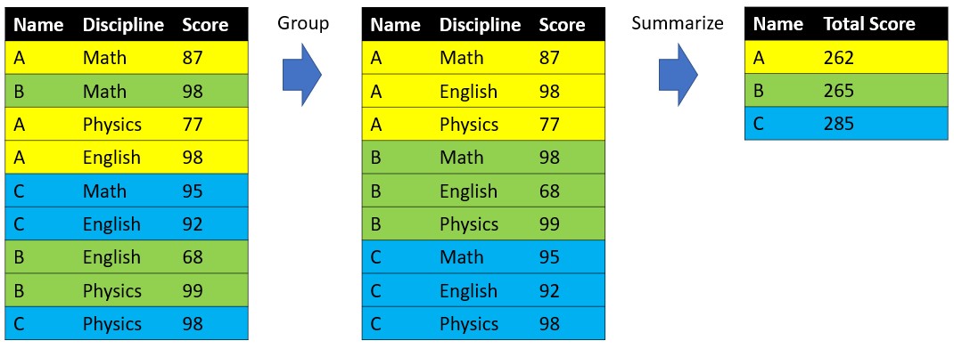
dataset %>%
  group_by(Name) %>%
  summarise(TotalSocre = sum(Score))
When it comes to our Minneapolis ACS dataset, we can use the combination of group_by() and summarise() to help use with many tasks.
minneapolis %>%
  group_by(YEAR) %>%  ## aggregate the data based on YEAR
  summarise(count = n(), ## number of respondents in each year
            AvgInc = mean(INCTOT, na.rm = T)) ## average personal income in each year
## # A tibble: 10 x 3
## YEAR count AvgInc
## * <int> <int> <dbl>
## 1 2010 2131 37605.
## 2 2011 2431 36715.
## 3 2012 2517 33152.
## 4 2013 2549 37392.
## 5 2014 2545 37238.
## 6 2015 2524 40902.
## 7 2016 2744 42901.
## 8 2017 2857 46994.
## 9 2018 2673 45557.
## 10 2019 2564 48519.minneapolis %>%
mutate(
RACE = case_when( ## change RACE from numeric values to racial categories
RACE == 1 ~ 'White',
RACE == 2 ~ 'African American',
RACE == 3 ~ 'Other'
)
) %>%
group_by(YEAR, RACE) %>% ## aggregate the data based on YEAR and RACE
summarise(MaxInc = max(INCTOT, na.rm = T)) ## maximum personal income for different racial groups in each year## # A tibble: 30 x 3
## # Groups: YEAR [10]
## YEAR RACE MaxInc
## <int> <chr> <dbl>
## 1 2010 African American 173200
## 2 2010 Other 362000
## 3 2010 White 637000
## 4 2011 African American 376000
## 5 2011 Other 200000
## 6 2011 White 594000
## 7 2012 African American 116000
## 8 2012 Other 396000
## 9 2012 White 461000
## 10 2013 African American 398000
## # ... with 20 more rows5.6 join()
We could use join() to do the same work of merge().
Name <- c('A', 'B', 'C') # create variable Name
MathScore <- c(87, 98, 95) # create variable Score1
df1 <- data.frame(Name, MathScore) # combine the variables into one data frame
df1
## Name MathScore
## 1 A 87
## 2 B 98
## 3 C 95Name <- c('B', 'D', 'C', 'A') # create variable Name
PhysicsScore <- c(99, 66, 98, 77) # create variable Score2
df2 <- data.frame(Name, PhysicsScore) # combine the variables into one data frame
df2## Name PhysicsScore
## 1 B 99
## 2 D 66
## 3 C 98
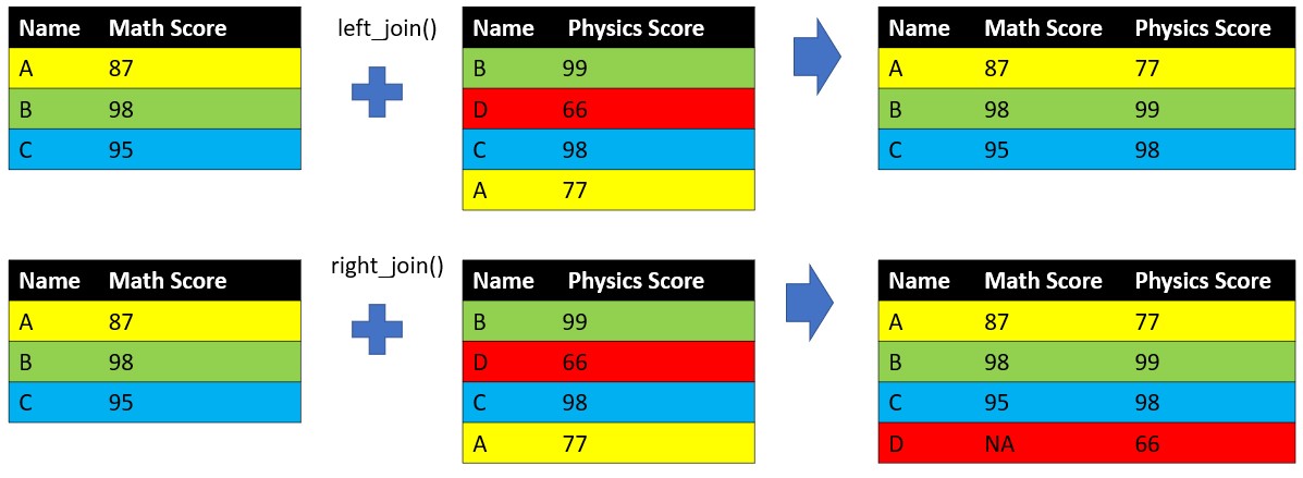
## 4 A 77df1 %>%
left_join(df2, by = 'Name')## Name MathScore PhysicsScore
## 1 A 87 77
## 2 B 98 99
## 3 C 95 98df1 %>%
right_join(df2, by = 'Name')## Name MathScore PhysicsScore
## 1 A 87 77
## 2 B 98 99
## 3 C 95 98
## 4 D NA 66Could you tell the difference between left_join() and right_join()?
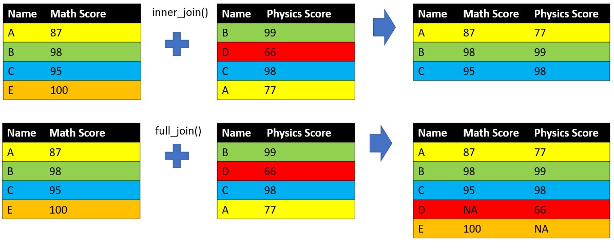
Besides left_join() and right_join(), we have inner_join() (keep only matched observations of two data frames) and full_join() (keep all observations of two data frames).
The codes below joins the poverty threshold dataset to the Minneapolis ACS dataset.
## import poverty threshold dataset
poverty <- read.csv('poverty.csv')

head(poverty, 10)
## YEAR THRESHOLD
## 1 2010 11139
## 2 2011 11484
## 3 2012 11720
## 4 2013 11888
## 5 2014 12071
## 6 2015 12082
## 7 2016 12228
## 8 2017 12488
## 9 2018 12784
## 10 2019 13011The poverty threshold dataset lists the poverty threshold in terms of personal income in the US from 2010 to 2019. The data was retrieved from this link
## join the poverty threshold dataset to the Minneapolis ACS dataset based on YEAR
minneapolis %>%
  left_join(poverty, by = 'YEAR') %>%
  head(10)
## YEAR SEX AGE RACE HISPAN EDUC EMPSTAT INCTOT FTOTINC THRESHOLD
## 1 2010 2 59 1 0 10 1 33100 49100 11139
## 2 2010 2 29 1 0 10 1 16000 49100 11139
## 3 2010 1 54 2 0 7 3 1100 NA 11139
## 4 2010 2 47 2 0 5 2 4800 4800 11139
## 5 2010 1 59 2 0 10 2 0 4800 11139
## 6 2010 2 10 2 0 1 0 NA 4800 11139
## 7 2010 1 24 1 0 5 1 15000 15000 11139
## 8 2010 1 26 2 3 6 1 18000 18000 11139
## 9 2010 1 51 1 0 6 1 35200 74400 11139
## 10 2010 2 47 1 0 6 1 39200 74400 11139Sometimes, people from different groups may give the same variables with different variable names. In this case, you may need to change the codes a little bit.
minneapolis %>%
  rename(TIME = YEAR) %>% ## rename the YEAR to TIME
  left_join(poverty, by = c('TIME' = 'YEAR')) %>% ## join the data based on different column names
  head(10)
## TIME SEX AGE RACE HISPAN EDUC EMPSTAT INCTOT FTOTINC THRESHOLD
## 1 2010 2 59 1 0 10 1 33100 49100 11139
## 2 2010 2 29 1 0 10 1 16000 49100 11139
## 3 2010 1 54 2 0 7 3 1100 NA 11139
## 4 2010 2 47 2 0 5 2 4800 4800 11139
## 5 2010 1 59 2 0 10 2 0 4800 11139
## 6 2010 2 10 2 0 1 0 NA 4800 11139
## 7 2010 1 24 1 0 5 1 15000 15000 11139
## 8 2010 1 26 2 3 6 1 18000 18000 11139
## 9 2010 1 51 1 0 6 1 35200 74400 11139
## 10 2010 2 47 1 0 6 1 39200 74400 11139rename() can help rename the column name in the data frame.
5.7 pivot_wider() and pivot_longer() in tidyr
We can categorize the data frame into two types. One is long data, the other is wide data. In the long form, each row is a score of one discipline for one student. In the wide form, each row contains the scores of all three disciplines for one student.
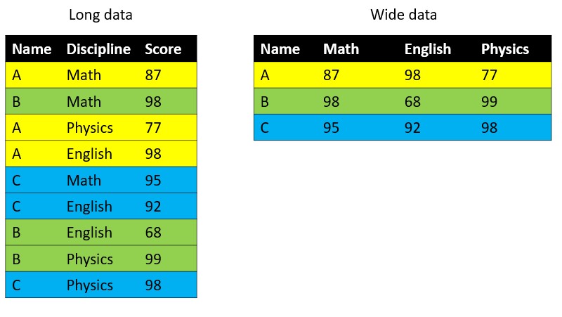
The long form and wide form data can be transformed to each other. We will use the example below as an illustration.
max_income <- minneapolis %>%
    mutate(
    RACE = case_when( ## change RACE from numeric values to racial categories
      RACE == 1 ~ 'White',
      RACE == 2 ~ 'African American',
      RACE == 3 ~ 'Other'
    )
  ) %>%
  group_by(YEAR, RACE) %>% ## aggregate the data based on YEAR and RACE
  summarise(MaxInc = max(INCTOT, na.rm = T)) ## maximum personal income for different racial groups in each year

head(max_income, 10)
## # A tibble: 10 x 3
## # Groups: YEAR [4]
## YEAR RACE MaxInc
## <int> <chr> <dbl>
## 1 2010 African American 173200
## 2 2010 Other 362000
## 3 2010 White 637000
## 4 2011 African American 376000
## 5 2011 Other 200000
## 6 2011 White 594000
## 7 2012 African American 116000
## 8 2012 Other 396000
## 9 2012 White 461000
## 10 2013 African American 398000We will use pivot_wider() and pivot_longer() in tidyr package to do the task.
## import the package
library(tidyr)
## from long to wide
wide_data <- max_income %>%
pivot_wider(names_from = RACE, values_from = MaxInc)
wide_data## # A tibble: 10 x 4
## # Groups: YEAR [10]
## YEAR `African American` Other White
## <int> <dbl> <dbl> <dbl>
## 1 2010 173200 362000 637000
## 2 2011 376000 200000 594000
## 3 2012 116000 396000 461000
## 4 2013 398000 398000 867000
## 5 2014 278000 459000 742000
## 6 2015 477000 513000 557000
## 7 2016 245000 469000 681000
## 8 2017 120000 503000 731000
## 9 2018 487000 337000 552000
## 10 2019 193000 495000 831000## from wide to long
wide_data %>%
pivot_longer(cols = `African American`:White, names_to = 'RACE', values_to = 'MaxInc')## # A tibble: 30 x 3
## # Groups: YEAR [10]
## YEAR RACE MaxInc
## <int> <chr> <dbl>
## 1 2010 African American 173200
## 2 2010 Other 362000
## 3 2010 White 637000
## 4 2011 African American 376000
## 5 2011 Other 200000
## 6 2011 White 594000
## 7 2012 African American 116000
## 8 2012 Other 396000
## 9 2012 White 461000
## 10 2013 African American 398000
## # ... with 20 more rows